Time Series Causal Graph

The class TimeSeriesCausalGraph, inheriting directly from CausalGraph, extends causal graphs to time series data.

For the theoretical background of causality for time series, please refer to Chapter 10 of Peters, J., Janzing, D. and Schölkopf, B., 2017. Elements of causal inference: foundations and learning algorithms (p. 288). The MIT Press.

The main addition of TimeSeriesCausalGraph lies in representing the time information in each node. The new TimeSeriesNode class inherits from the corresponding Node and keeps all original properties:

• identifier
• variable_type

The TimeSeriesNode class has two additional properties:

• time_lag: the time difference with respect to the reference time 0.
• variable_name: the name of the variable (without the lag information).

The TimeSeriesNode can be instantiated as follows:

from cai_causal_graph.graph_components import TimeSeriesNode

# Via identifier
ts_node = TimeSeriesNode(identifier='X lag(n=1)')

# Via time lag and variable name
ts_node = TimeSeriesNode(time_lag=-1, variable_name='X')

However, it is easier to just add nodes directly to the TimeSeriesCausalGraph.

The format of the identifier is the following:

• f'{variable_name}' if time_lag == 0
• f'{variable_name} lag(n={time_lag})' if time_lag < 0
• f'{variable_name} future(n={time_lag})' if time_lag > 0

Examples of time series causal graphs

The following examples have been drawn from Peters, J., Janzing, D. and Schölkopf, B., 2017. Elements of causal inference: foundations and learning algorithms (p. 288). The MIT Press.

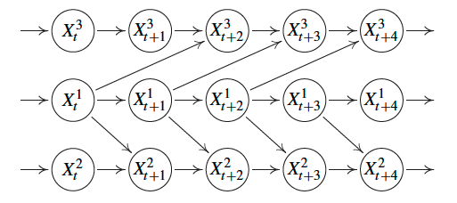
Example of a time series causal graph with no instantaneous effects, i.e., no edges between nodes at the same time stamp.

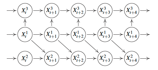
Example of a time series causal graph with instantaneous effects, i.e., there are edges between nodes at the same time stamp.

Summary graph of the full time series causal graphs above.

Construction

Direct initialization

You can instantiate a TimeSeriesCausalGraph directly using its constructor.

from cai_causal_graph import EdgeType, TimeSeriesCausalGraph

ts_cg = TimeSeriesCausalGraph()
# Nodes are added automatically if they are not in the graph when an edge is added.
ts_cg.add_edge('X1 lag(n=1)', 'X1', edge_type=EdgeType.DIRECTED_EDGE)
ts_cg.add_edge('X2 lag(n=1)', 'X2', edge_type=EdgeType.DIRECTED_EDGE)
ts_cg.add_edge('X1', 'X3', edge_type=EdgeType.DIRECTED_EDGE)

From a CausalGraph

Alternatively, you can instantiate a TimeSeriesCausalGraph from a CausalGraph instance. If the nodes are named correctly, the time information will be extracted accordingly.

from cai_causal_graph import CausalGraph, EdgeType, TimeSeriesCausalGraph

cg = CausalGraph()
cg.add_edge('X1 lag(n=1)', 'X1', edge_type=EdgeType.DIRECTED_EDGE)
cg.add_edge('X2 lag(n=1)', 'X2', edge_type=EdgeType.DIRECTED_EDGE)
cg.add_edge('X1', 'X3', edge_type=EdgeType.DIRECTED_EDGE)

ts_cg = TimeSeriesCausalGraph.from_causal_graph(cg)

The TimeSeriesCausalGraph will have the same nodes and edges as the CausalGraph, but will be aware of the time information so 'X1 lag(n=1)' and 'X1' represent the same variable but at different times.

From an adjacency matrix

You can instantiate a TimeSeriesCausalGraph from an adjacency matrix and optionally a list of node names.

import numpy
from cai_causal_graph import TimeSeriesCausalGraph

# The adjacency matrix should be a squared binary numpy array
adjacency_matrix: numpy.ndarray

# Simply via the adjacency matrix
ts_cg = TimeSeriesCausalGraph.from_adjacency_matrix(adjacency=adjacency_matrix)

# Also specifying the node names
ts_cg = TimeSeriesCausalGraph.from_adjacency_matrix(
    adjacency=adjacency_matrix, node_names=['X1 lag(n=1)', 'X1', 'X2 lag(n=1)', 'X2', 'X3']
)

From multiple adjacency matrices

You can instantiate a TimeSeriesCausalGraph from a dictionary of adjacency matrices, where the keys are the time deltas. For example, the adjacency matrix with time delta -1 is stored in adjacency_matrices[-1] as would correspond to X-1 -> X, where X is the set of nodes.

import numpy
from cai_causal_graph import TimeSeriesCausalGraph

adjacency_matrices = {
    -2: numpy.array([[0, 0, 0], [1, 0, 0], [0, 0, 1]]),
    -1: numpy.array([[0, 1, 0], [1, 0, 0], [0, 0, 0]]),
    0: numpy.array([[0, 1, 1], [0, 0, 1], [0, 0, 0]]),
}

# Simply via the adjacency matrices
ts_cg = TimeSeriesCausalGraph.from_adjacency_matrices(adjacency_matrices=adjacency_matrices)

# Also specifying the variable names
ts_cg = TimeSeriesCausalGraph.from_adjacency_matrices(adjacency_matrices=adjacency_matrices, variable_names=['X', 'Y', 'Z'])

Query the nodes and the variables

You can extract all the variable names from the nodes of the TimeSeriesCausalGraph.

from cai_causal_graph import TimeSeriesCausalGraph

ts_cg: TimeSeriesCausalGraph

# Return a list of variable names from a list of node names
node_names = ['X', 'X lag(n=1)', 'Y', 'Z lag(n=2)']
ts_cg.get_variable_names_from_node_names(node_names)
# This will return ['X', 'Y', 'Z']

Conversely, you can extract a list of TimeSeriesNodes in the graph from a given list of identifiers.

from typing import List
from cai_causal_graph import TimeSeriesCausalGraph
from cai_causal_graph.graph_components import TimeSeriesNode

ts_cg: TimeSeriesCausalGraph

# A single node (it will be a list with one element)
variable: List[TimeSeriesNode] = ts_cg.get_nodes(identifier='X lag(n=1)')

# Multiple nodes
variables: List[TimeSeriesNode] = ts_cg.get_nodes(identifier=['X', 'X lag(n=1)'])

Add nodes

You can add a TimeSeriesNode to the TimeSeriesCausalGraph.

from cai_causal_graph import NodeVariableType, TimeSeriesCausalGraph
from cai_causal_graph.graph_components import TimeSeriesNode

ts_cg: TimeSeriesCausalGraph

# Via a node object
new_node = TimeSeriesNode(time_lag=-3, variable_name='X')
ts_cg.add_node(node=new_node)

# Via identifier
ts_cg.add_node(identifier='X lag(n=3)')

# Via variable name and time lag
ts_cg.add_node(variable_name='X', time_lag=-33)

# Variable type can also be specified
ts_cg.add_node(identifier='X lag(n=3)', variable_type=NodeVariableType.CONTINUOUS)

Add edges

You can add time series edges to the TimeSeriesCausalGraph.

from cai_causal_graph import EdgeType, TimeSeriesCausalGraph

ts_cg: TimeSeriesCausalGraph

# Via identifier (the edge type can be specified if desired)
ts_cg.add_edge(source='X lag(n=3)', destination='Y lag(n=3)', edge_type=EdgeType.DIRECTED_EDGE)

# Add edge by pair (the edge type can be specified if desired)
ts_cg.add_edge_by_pair(pair=('X lag(n=2)', 'Y lag(n=2)'), edge_type=EdgeType.DIRECTED_EDGE)

# Add multiple edges by specifying tuples of source and destination node identifiers and with default setup
ts_cg.add_edges_from(pairs=[('X lag(n=2)', 'Y lag(n=2)'), ('X lag(n=3)', 'Y lag(n=3)')])

# Via time edge
ts_cg.add_time_edge(source_variable='X', source_time=-2, destination_variable='Y', destination_time=-2, edge_type=EdgeType.DIRECTED_EDGE)

Replace nodes

Replace a node in the TimeSeriesCausalGraph.

from cai_causal_graph import NodeVariableType, TimeSeriesCausalGraph

ts_cg: TimeSeriesCausalGraph

# Via identifier
ts_cg.replace_node(node_id='X lag(n=3)', new_node_id='Y lag(n=3)')
# Via variable name and time lag
ts_cg.replace_node(node_id='X lag(n=3)', time_lag=3, variable_name='Y')

# Variable type can also be specified
ts_cg.replace_node(node_id='X lag(n=3)', new_node_id='Y lag(n=3)', variable_type=NodeVariableType.CONTINUOUS)

Delete nodes and edges

You can delete nodes and edges from the TimeSeriesCausalGraph.

from cai_causal_graph import EdgeType, TimeSeriesCausalGraph

ts_cg: TimeSeriesCausalGraph

# Delete node
ts_cg.delete_node(identifier='X lag(n=3)')

# Delete edge (the edge type can be specified if desired)
ts_cg.delete_edge(source='X lag(n=3)', destination='Z lag(n=3)', edge_type=EdgeType.DIRECTED_EDGE)

# Delete edge from pair (the edge type can be specified if desired)
ts_cg.remove_edge_by_pair(pair=('X lag(n=3)', 'Z lag(n=3)'), edge_type=EdgeType.DIRECTED_EDGE)

Minimal graph

The minimal graph is the graph with the minimal number of edges that is equivalent to the original graph. In other words, it is a graph that has no edges whose destination is not time delta 0.

from cai_causal_graph import TimeSeriesCausalGraph

ts_cg: TimeSeriesCausalGraph

# Check whether a graph is in its minimal form
# Returns True if the graph is a minimal graph, False otherwise
is_minimal = ts_cg.is_minimal_graph()

# Get the minimal graph
minimal_graph: TimeSeriesCausalGraph = ts_cg.get_minimal_graph()

Summary graph

You can collapse the graph in time into a single node per variable (column name). This can become cyclic and bi-directed as X(t-1) -> Y and Y(t-1) -> X would become X <-> Y. Note that the summary graph is a CausalGraph object.

from cai_causal_graph import CausalGraph, TimeSeriesCausalGraph

ts_cg: TimeSeriesCausalGraph

summary_graph: CausalGraph = ts_cg.get_summary_graph()

Stationary graph

It may be useful to check whether the TimeSeriesCausalGraph is stationary, i.e., its edges are not dependent on the corresponding time lags. In other words, the graph is the same for all time lags.

Stationarity is a useful concept for future prediction: if the graph is stationary, it can be used to predict the future for any time lag. Conversely, if the graph is not stationary, it can only be used to predict the future for the specified time lags. Thus, in a stationary graph, if the edge X lag(n=1) -> Y lag(n=1) exists, also the edge X lag(n=2) -> Y lag(n=2) must be present if the nodes X lag(n=2) and Y lag(n=2) are in the graph.

from cai_causal_graph import TimeSeriesCausalGraph

ts_cg: TimeSeriesCausalGraph

# Check whether a graph is stationary
# Returns True if the graph is a stationary, False otherwise
is_stationary = ts_cg.is_stationary_graph()

# Get the stationary graph
stationary_graph: TimeSeriesCausalGraph = ts_cg.get_stationary_graph()

note

It is important to note that the minimal graph is not necessarily stationary. Therefore, the underlying process defined in the minimal graph does not need to be stationary, but if the minimal graph is non-stationary it does not always mean that the process is not stationary. It may only mean that the graph is missing at least one of the corresponding edges in time. This is the more likely scenario. Please see the example below of a minimal graph that is not stationary as it is missing the edge X1 lag(n=1) -> X2 lag(n=1). Adding that edge would make the graph no longer minimal so the process may be stationary, but obviously the minimal graph will be non-stationary. The stationary graph is obtained by extending (in time) the minimal graph with all the edges to the correct backward and forward time lags.

Extended graph

You can extend the graph in time by adding nodes for each variable at each time step from backward_steps to forward_steps. If a backward step of n is specified, it means that the graph will be extended in order to include nodes back to time -n and all the nodes connected to them as specified by the minimal graph. An extra include_all_parents flag can be set so that, in addition to all nodes as far back as backward_steps, extra nodes and edges will be added as far back that all nodes up to backward_steps in the past have all their parents and inbound edges. This means that the extended graph may now have nodes at lags further back than backward_steps. If a forward step of n is specified, it means the graph will be extended in order to include nodes forward to time n and all the nodes connected to them as specified by the minimal graph. include_all_parents is only valid when specifying a backward_steps, and will have no effect on the logic of forward_steps. If both backward_steps and forward_steps are None, the original graph is returned.

from cai_causal_graph import TimeSeriesCausalGraph

ts_cg: TimeSeriesCausalGraph
backward_steps = 2
forward_steps = 3

extended_graph = ts_cg.extend_graph(backward_steps=backward_steps, forward_steps=forward_steps)

# With all parents
extended_graph = ts_cg.extend_graph(backward_steps=backward_steps, forward_steps=forward_steps, include_all_parents=True)

Other methods

For all the other base properties and methods, please refer to the documentation of CausalGraph, from which TimeSeriesCausalGraph inherits.

Example

You define the following as the initial TimeSeriesCausalGraph instance. Please note that this graph is stationary.

If you query for the minimal graph, you will get the following:

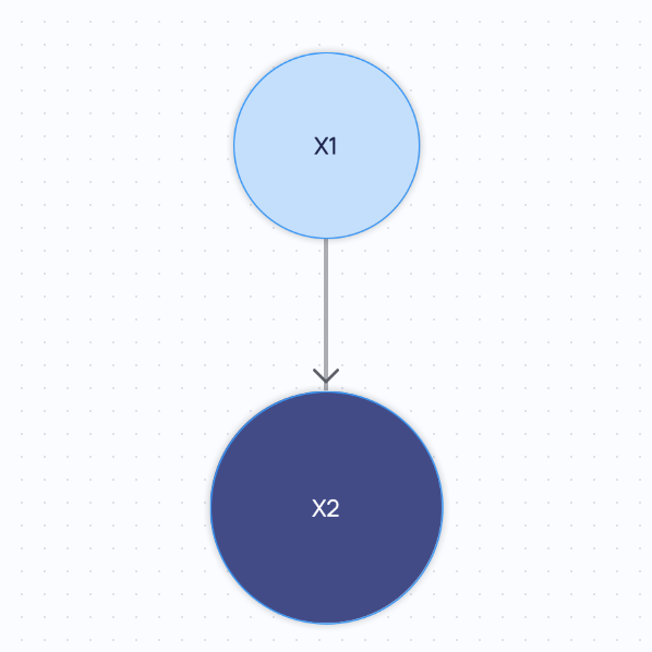
If you query for the summary graph, you will get the following:

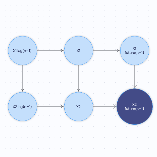
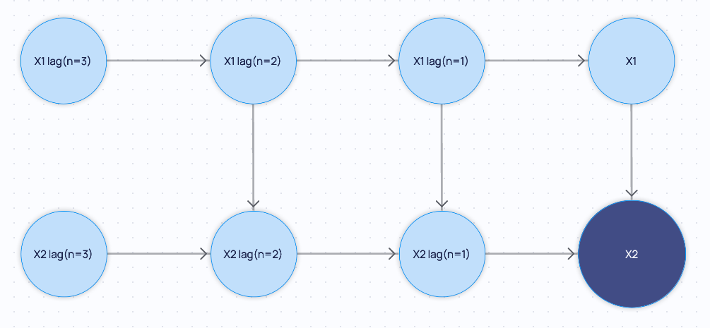
If you extend the minimal graph backward_steps=2 and forward_steps=0 with default arguments:

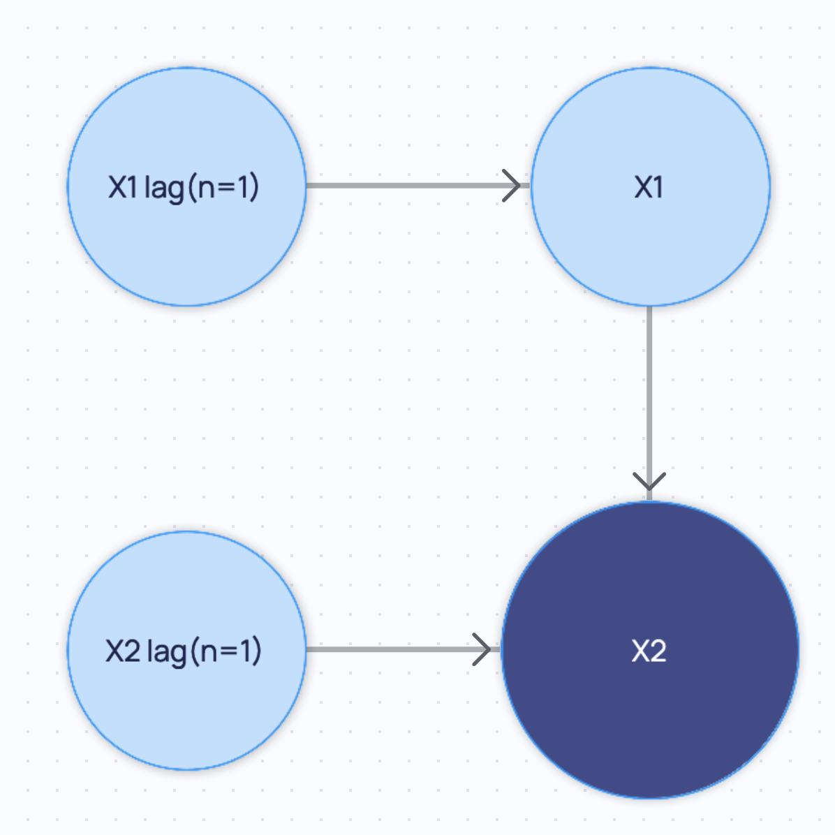
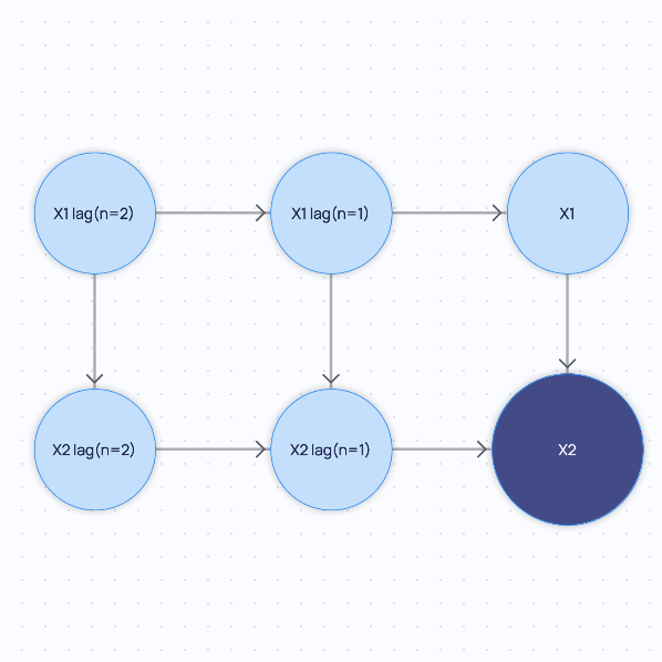
Finally, if you extend the minimal graph with backward_steps=2 and forward_steps=0 but setting include_all_parents=True:

Markov Equivalence Classes

Certain causal relationships yield the same conditional independencies and are therefore indistinguishable from each other with only observational data. The set of such causal relationships is called the Markov Equivalence Class (MEC) for a particular set of nodes. Most causal discovery methods that use observational data are only able to return the MEC of a set of nodes and not the full directed acyclic graph (DAG).

One prominent representation of MECs is a Completed Partially Directed Acyclic Graph (CPDAG), which only contains directed (->) and undirected (--) edges. In this case, an undirected edge simply implies that a causal relationship can point either way, i.e. A -- B can be resolved to either A -> B or A <- B.

A Partial Ancestral Graph (PAG) can encode all the information that CPDAGs can, but also provides more detailed information about the relationships between variables, such as including whether a latent confounder is likely to exist or selection bias is likely to be present.

Specifically, in addition to directed edges (A -> B or A <- B) and undirected edges (A -- B), PAGs represent an equivalence class of MAGs (Maximal Ancestral Graphs) that may also contain bi-directed edges A <-> B, which implies that there is a latent confounder between the respective variables. They also introduce the additional "wild-card" or "circle" edges A -o B, which can either be a directed or undirected arrow head, i.e. A -o B can be resolved to A -- B or A -> B.

MAGs and PAGs retain the pairwise Markov property of DAGs - every missing edges corresponds to a statement of conditional independence amongst the observed variables. Contrary to DAGs, however, the presence of an edge does not mean necessarily that two nodes are adjacent in the (presumed) true DAG - which may include unobserved variables. Rather, it simply means that a conditional set that separates the two nodes could not be found amongst the observed variables.

Similar to a CPDAG, a PAG can represent a number of DAGs. Therefore, PAGs, MAGs, CPDAGs and DAGs can be thought of in a hierarchical way.

All these edge types can be represented by EdgeType and edges of these types can be added to the TimeSeriesCausalGraph (as shown above) as long as the ordering of time is respected.

In addition to DAGs (as shown above), the TimeSeriesCausalGraph also supports Markov equivalence classes, as in the following example with a PAG.

from cai_causal_graph import EdgeType, TimeSeriesCausalGraph

ts_cg = TimeSeriesCausalGraph()

ts_cg.add_edge('X1 lag(n=1)', 'X1', edge_type=EdgeType.DIRECTED_EDGE)
ts_cg.add_edge('X1 lag(n=1)', 'X2', edge_type=EdgeType.UNKNOWN_DIRECTED_EDGE)